I’m super excited that the Melbourne Kotlin meetup is back after a COVID-induced hiatus, and I’m just as excited to be presenting!

Come down to the Block-AfterPay offices at 6pm on August 11 to hear Zenab Bohra present “Introduction to FP in Kotlin”, and I’ll be talking about “Embedding Golang in a Kotlin app: how to do it and why you shouldn’t”.

For more details, and to RSVP, check out the August meetup page.

Update: the recording of both talks are now available on YouTube. Zenab’s talk begins at 3:34, and my talk starts at 45:00.

I’m constantly asking myself a bunch of questions to help improve Batect: are Batect’s users having a good experience? What’s not working well? How are they using Batect? What could Batect do to make their lives easier?

I first released Batect back in 2017. Since then, the userbase has grown from a handful of people that could fit around a single desk to hundreds of people all over the globe.

Back when everyone could fit around a desk, answering these questions was easy: I could stand up, walk over to someone, and ask them. (Or, if I was feeling particularly lazy, I could stay seated and ask over the top of my screen.)

But with this growth, now I have another question: how do I break out of my bubble and feedback and ideas from those I don’t know?

This is where telemetry data comes into the picture. Besides signals like GitHub issues, discussions, suggestions and the surveys I occasionally run, telemetry data has been invaluable to help me get a broader understanding of how users use Batect, the problems they run into and the environments they use Batect in. This in turn has helped me prioritise the features and improvements that will have the greatest impact, and design them in a way that will be the most useful for Batect’s users.

In this (admittedly very long) post, I’m going to talk through what I mean by telemetry data, how I went about designing the telemetry collection system, Abacus, and finish off with two stories of how I’ve used this data.

• Telemetry?
• Key design considerations
• The design
• Examples of where I’ve used this data
  • Shell tab completion
  • Renovate
• What works well, and what doesn’t
• In closing

Telemetry?

Similar to Honeycomb’s definition of observability for production systems, I wanted to be able to answer questions about Batect and it’s users I haven’t even thought of yet, and do so without having to make any code changes and push out a new version of Batect.

This is exactly the problem that Batect’s telemetry data solves. Every time Batect runs, it collects information like:

• what version of Batect you’re using
• what operating system you’re using
• what version of Docker you’re using
• a bunch of other interesting environmental information (what shell you use, whether you’re running Batect on a CI runner or not, and more)
• data on the size of your project
• what features you are or aren’t using
• notable events such as if an update nudge was shown, or if an error occurred
• timing information for performance-critical operations such as loading your configuration file

…and more! There’s a full list of all the data Batect collects in its privacy policy.

With this data, I can answer all kinds of questions. Here are just a few real examples:

• How long does it take for new versions of Batect to be adopted? (answer: anywhere from hours to months, depending on the user)
• How many times does a user see an update nudge before they update Batect? (answer: lots - some users even seem to never respond to these)
• Does using BuildKit really make a difference to image build times? (answer: yes)
• Could adding shell tab completion really be useful? (answer: yes, humans make lots of typos)
• Was adding shell tab completion actually useful? (answer: yes, it prevents lots of typos)
• What’s the common factor behind this odd error that only a handful of users are seeing? (answer: one particular version of Docker)

Key design considerations

There were a couple of key aspects I was considering as I sketched out what the telemetry collection system could look like, in rough priority order:

• Privacy and security: given the situations and environments where Batect is used, preserving users’ and organisations’ security and privacy are critical. This is not only because it’s simply the right thing to do, but because any issues here would likely lead to a loss of trust and to them blocking telemetry data or not using Batect, which is obviously not what I want.

• User experience impact: Batect is part of developers’ core feedback loop, and so any changes that made it noticeably less reliable or less performant were non-starters.

• Cost: any expense to build or run the system would be coming out of my own pocket, so minimising the cost was important to me.

• Ease of maintenance: this is something I largely maintain in my own time, so minimising the amount of ongoing care and feeding was another high priority. Another aspect of maintenance was also designing something simple and easy to understand, so that when I come back to do any future maintenance, I wouldn’t need to spend a lot of time re-learning a tool, service or library.

• Flexibility: I want to be able to investigate new ideas and answer questions I haven’t thought of yet, as well as expand the data I’m collecting as Batect evolves, and so I needed a system that supports these goals.

• Learning: given I was building this on my own time, I also wanted to use this as an opportunity to learn more about a few technologies and techniques I hadn’t used much before.

The design

It’s probably easiest to understand the overall design of the system by following the lifecycle of a single session.

Diagram showing main components in the system and steps in data flow (click to enlarge)

A session represents a single invocation of Batect - so if you run ./batect build and then ./batect unitTest, this will create two telemetry sessions, one for each invocation.

1️⃣ As Batect runs, it builds up the session, recording details about Batect, the environment it’s running in and your configuration, amongst other things. It also records particular events that occur, like when an error occurs or when it shows you a “new version available” nudge, and captures timing spans for performance-sensitive operations like loading configuration files.

Just before Batect terminates, it writes this session to disk in the upload queue, ready to be uploaded in a future invocation.

2️⃣ When Batect next runs, it will launch a background thread to check for any outstanding telemetry sessions waiting in the upload queue.

3️⃣ Any outstanding sessions are uploaded to Abacus. Once each upload is confirmed as successful, the session is removed from disk.

4️⃣ Once Abacus receives the session, it performs some basic validation and writes the session to a Cloud Storage bucket. Each session is assigned a unique UUID by Batect when it is created, so Abacus uses this ID to deduplicate sessions if required.

5️⃣ Once an hour, a BigQuery Data Transfer Service job checks for new sessions in the Cloud Storage bucket and writes them to a BigQuery table.

6️⃣ With the data now in BigQuery, I can either perform ad-hoc queries over the data to answer specific questions, or use Google’s free Data Studio to visualise and report on the data.

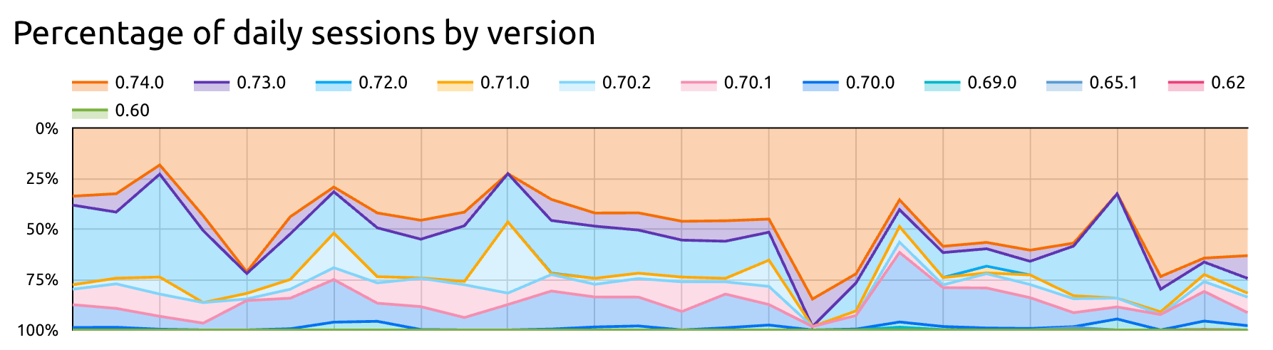
For example, I can report on what version of Batect is being used:

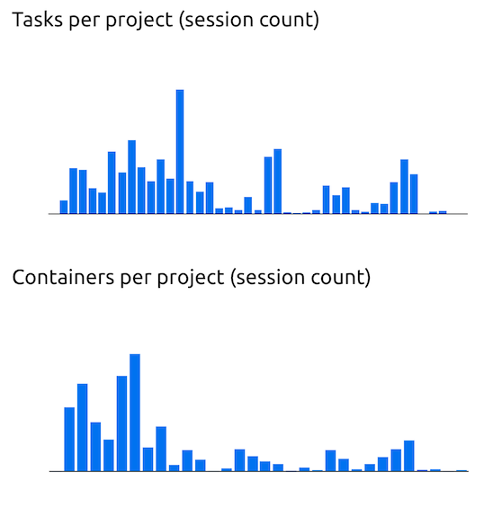
Or the distribution of the number of tasks and containers in each project:

There a bunch of other important details I’ve skipped over here in the interest of brevity - topics like not collecting personally identifiable information, or even potentially-identifiable information and managing consent - but these are all important aspects to consider if you’re thinking of building a similar system yourself.

Examples of where I’ve used this data

Some of my favourite stories of how I’ve used this data are for prioritising Batect’s shell tab completion functionality and validating that it had the intended impact, and for prioritising contributing support for Batect to Renovate.

Shell tab completion

Batect’s main user interface is the command line: to run a task, you execute a command like ./batect build or ./batect test from your shell. One of the most frequently-requested features was support for shell tab completion, so that instead of typing out build or test, you could type just the first letter or two, press Tab, and the rest of the task name would be completed for you.

While I could definitely see the value in this, I was worried I was over-emphasising features I’d like to see based on how I usually work and interact with applications, and wanted to confirm that this would actually be valuable for a large portion of Batect’s userbase. I formed a hypothesis that shell tab completion would help reduce the number of sessions that fail because the task name cannot be found, likely because of a typo.

So, I turned to the data I had and found that roughly 2.6% of sessions fail because the task cannot be found. This seemed very high and was enough for me to feel confident investing some time and effort implementing shell tab completion.

Of course, the next question was which shell to focus on first: Bash? Zsh? My personal favourite, Fish? My gut told me most people would likely be using Zsh or Bash as their default shell, but here the data told a different story: the shells used most commonly by Batect’s users are actually Fish and Zsh. So that’s where I started - I added tab completion functionality for both Fish and Zsh - and, thanks to the data I had, I was able to prioritise my limited time to focus on the shells that would help the largest number of users.

And, thanks once again to telemetry data, once I’d released this feature, I was also able to quickly validate my hypothesis: users that use shell tab completion experience “task not found” errors over 30% less than those that don’t use it.

Renovate

Batect is driven by the batect and batect.cmd wrapper scripts that you drop directly into your project and commit alongside your code.

Most of the time, this is great: you can just clone a repository and start using it without needing to install anything, and you can be confident everyone on your team is using exactly the same version.

However, there’s a drawback hiding in the last part of that sentence: this design also means that you or one of your teammates must upgrade the wrapper script to use a new version of Batect. Based on both anecdotal evidence from users asking for features that already existed, as well as telemetry data, I could see that many teams were not upgrading regularly. And from telemetry data, I also knew this was happening even while users were seeing an upgrade nudge like this many hundreds of times a day:

Version 0.79.1 of Batect is now available (you have 0.74.0).
To upgrade to the latest version, run './batect --upgrade'.
For more information, visit https://github.com/batect/batect/releases/tag/0.79.1.

Armed with this information, I decided to try to help users upgrade more often and more rapidly - there was little point spending time building new features and fixing bugs if only a small proportion of users benefited from these improvements.

My solution was to add support for Batect’s wrapper script to Renovate. This means that projects that use Renovate will automatically receive pull requests to upgrade to the new version whenever I release a new version of Batect, and upgrading is as simple as merging the PR.

Again, the data shows this has been a success: whereas previously, a new version would only slowly be adopted, now, new versions of Batect make up over 40% of sessions within a month of release.

What works well, and what doesn’t

The Abacus API is a single Golang application deployed as a container to GCP’s Cloud Run. I’ve been really happy with Cloud Run: it just works. My only wish is that it had better built-in support for gradual rollouts of new versions. This is something that can be done with Cloud Run, but as far as I can tell, it requires some form of external orchestration to monitor the new version and adjust the proportion of traffic going to the new and old versions as the rollout progresses.

Cloud Run also integrates nicely with GCP’s monitoring tooling. I wasn’t sure about using GCP’s monitoring tools at first - I was expecting that I’d quickly run into a variety of limitations and rough edges like with AWS’ CloudWatch suite - but I’ve been pleasantly surprised. For something of this scale, the tools more than meet my needs, and I haven’t felt the need to consider any alternatives. I recently added Honeycomb integration, but this was more out of curiousity and wanting to learn more about Honeycomb than a need to use another tool.

The pattern of dropping session data into Cloud Storage to be synced by BigQuery Transfer Service into BigQuery has also been more than sufficient for my needs. While this does introduce a delay of up to two hours between data being received and it being ready to query in BigQuery, I rarely want to query data so rapidly, and the alternative of streaming data would be both more complex and more costly.

All of this also almost fits within GCP’s free tier: the only item that regularly exceeds the free allowance is upload operations to Cloud Storage, as each individual session is uploaded individually as a single object, and the free tier includes only 5,000 uploads per month. I could reduce this cost by batching sessions together and uploading a batch as a single file, but this would again introduce more complexity and cost for little benefit.

On the client side, the concept of the upload queue has been really successful: uploading sessions in the background of a future invocation minimises the user impact of uploading this data, and provides a form of resilience against any transient network or service issues. (If a session can’t be uploaded for some reason, Batect will try to upload it again next time, or give up once the session is 30 days old.)

The biggest area for improvement is how I manage reports and dashboards. I’m currently using Data Studio for this, and while it too largely just works, there are a couple of key features missing that I’d really like to see. For example, it’s not possible to version control the definition of a report, making changes risky, and doesn’t have built-in support for visualisations like histograms or heatmaps, limiting how I can visualise some kinds of data.

In closing

Collecting telemetry data is something I wish I’d added to Batect far earlier. But now that I have this rich data, I can’t imagine life without it. It’s helped me prioritise my limited time and enabled me to deliver a more polished product to users.

On top of this, I’ve achieved my design goals for Abacus, including preserving users’ privacy and minimising the performance impact of collecting this data. And I’ve learnt about services like BigQuery and Data Studio along the way.

If you’re interested in checking out the code for Abacus, it’s available on GitHub, as is the client-side telemetry library used by Batect.

Updated July 10 to include more details of the tools and services behind Abacus.

I’ve just published okhttp-system-keystore, a small library that makes it easy to use trusted certificates from the operating system keystore (Keychain on macOS, Certificate Store on Windows) with OkHttp.

Feedback, suggestions and ideas are welcome!

After quite a hiatus, I’m going to try to post here more regularly… let’s start with two topics close to my heart: Kotlin and Batect.

A fairly frequent question I get is: why is Batect written in Kotlin? And often the question behind the question is: why isn’t it written in Golang?

To answer those questions we need to go back in time to 2017, when I first started working on Batect.

I had the idea for what would become Batect after working with a couple of different teams who were all trying to use Dockerised development environments. And after going through the pain of trying to once again reinvent the same less-than-ideal setup we’d had on a previous team, I decided to build a proof of concept for my idea.

At the time, all I wanted to do was quickly build a proof of concept. I was more concerned about building it quickly and having fun and learning while I built it than anything else: I wasn’t expecting the proof of concept to be anything more than some throwaway code. (Famous last words.) I had been dabbling in Kotlin for a while and thought this would be a great opportunity to play with a language I really liked.

Fast forward a bit and we come to late 2017. I’d finished the proof of concept in Kotlin and demoed it to my team for feedback. They gave some really positive feedback and that encouraged me to seriously consider turning Batect into something more than a proof of concept.

At this point, I had a codebase that could run a sample project, a working interface to Docker that invoked the docker command to pull images, create containers etc., and some basic tests. I had two choices: continue with this largely working app, or throw it away and start afresh.

As part of considering whether or not to start afresh, I thought for a while about whether to continue in Kotlin or switch to Golang. There were four things that were going through my mind:

I had something that worked and a codebase that was in relatively good shape.

Switching to Golang would require starting from scratch. Given I was doing this entirely on my own time, that didn’t seem like a great use of time, especially for something that still didn’t have any active users.

The main argument in favour of Golang was the fact that the vast majority of the Docker ecosystem is written in Golang.

If Batect was written in Golang, I could take advantage of things such as the Docker client library for Golang, rather than write my own for Kotlin. I was using the docker CLI to communicate with the Docker daemon from Kotlin and changing to use the HTTP API didn’t seem that difficult if needed later.

Another argument in favour of Golang was the ability to build a single self-contained binary for distribution, rather than requiring users to install a JVM.

However, earlier that year, JetBrains had announced the first preview of Kotlin/Native, which would allow the same thing for Kotlin code. Younger, naïve-r me assumed that would be good enough and easy enough to adopt in the future should the use of a JVM really turn out to be a problem.

The last thing was simply personal preference and how much I enjoyed working with the language.

Again, this was something I was doing on my own time and had no active users yet, so personal enjoyment was one of the main priorities for me. At the time, I was working on a production Golang system and was finding the language somewhat lacking in comparison to Kotlin. Dependency management in Golang was a pain (this would be fixed with the introduction of modules in Go 1.11 in August the next year), and I found Kotlin’s syntax and type system enabled me to write expressive, safe code.

So I chose to continue in Kotlin.

Looking back on that decision, there are definitely some things that remain true today, and others where the situation turned out to be a bit different:

Not rewriting Batect from scratch meant I was able to continue adding new features and incorporating feedback. This meant that Batect was ready to introduce to a new team in late 2017. This team chose not only to take a risk and adopt a completely unproven tool, but continue to this day to be some of its strongest advocates. If I’d stopped to rewrite Batect in Golang, I would have missed that opportunity.

Using the docker CLI worked reasonably well for quite some time, but eventually the performance hit of spawning new processes to interact with the Docker daemon was starting to have a noticeable impact.

Switching to use the API directly was, sadly, not as straightforward as I hoped. In particular, I had failed to consider the client-side complexities of some of Docker’s features, such as connection configuration management, image registry credentials and managing the terminal while streaming I/O to and from the daemon.

This has played out over and over again, and has been a significant drain on my time, especially when it came to adding support for BuildKit, which is largely undocumented, requires extensive client-side logic to implement correctly and relies on a number of Golang idiosyncrasies.

Kotlin/Native sadly hasn’t matured as quickly as I expected. So Batect still requires a JVM, and this adds a small barrier to entry for some people. Having said that, JetBrains is still actively developing Kotlin/Native and significant progress has been made in the last 12 months or so, so I remain hopeful that removing the need for a JVM is still an achievable goal. This will not be painless – Batect has dependencies on some JVM-only libraries at the moment – but it certainly seems within reach.

The last point will always be a matter of personal opinion, but Kotlin remains my favourite language to this day.

Every now and then I question my choice and whether it was the right decision to continue building Batect in Kotlin. While some things may well have been easier had I chosen to use Golang, Batect has hundreds of active users who love using it, and I still enjoy working on it after all this time, and those are the two things that matter most to me.

Thank you to Andy Marks, Inny So and Jo Piechota for providing feedback on a draft version of this post.

Last month I spoke at ThoughtWorks Australia’s inaugural ‘Evolution by ThoughtWorks’ conference in Melbourne and Sydney, presenting on Build and testing environments as code: because life’s too short not too.

The slides and video from the talk are now available on the ThoughtWorks website.

The sample environment I used during the presentation is available on GitHub, and you can find more information about batect on its GitHub page.

Last night I spoke at the DevOps Melbourne meetup, presenting on Build and testing environments as code: because life’s too short not too.

The slides are available to download as a PDF, the sample environment I used during the presentation is available on GitHub, and you can find more information about batect on its GitHub page.

I’ve been talking quite a bit lately about Docker-based build environments (in Hamburg, in Munich, and at many of our clients).

One of the biggest drawbacks of the technique is the poor integration story for IDEs. Many IDEs require that your build environment (eg. target JVM and associated build tools) is installed locally to enable all of their useful features like code completion and test runner integration. But if this is isolated away in a container, the IDE can’t access it, so all these handy productivity features won’t work.

However, it looks like JetBrains in particular is starting to integrate these ideas into their products more:

• WebStorm will now allow you to configure a ‘remote’ Node.js interpreter in a local Docker image (details here)
• RubyMine takes this one step further: you can configure a Ruby interpreter based on a service definition in a Docker Compose file (details here). A similar feature is available for Python in PyCharm.

Both of these are great steps forward, and if you’re using Docker-based build environments, I’d encourage you to take a look at this.

Now, if only they’d do this for JVMs in IntelliJ…

Tonight I spoke at the ThoughtWorks Munich meetup, presenting an updated version of my presentation Docker’s not just for production: using containers for your development environment. There are two major changes over the previous version:

• I’ve added a section about using containers to manage test environments, in addition to the existing content about build environments
• I’ve reworked the structure of the presentation based on feedback to focus more on the technique itself rather than a discussion of existing alternatives

The slides are available to download as a PDF, and the sample environment I used during the presentation is available on GitHub.

Tonight I spoke at the ThoughtWorks Hamburg meetup, presenting Docker’s not just for production: using containers for your development environment.

The slides are available to download as a PDF, and the sample Docker-based development environment I used during the presentation is available on GitHub.

Over three months ago (yeah… sorry about that) we took a look at the linker script for the STM32F4 project template. I promised that we’d examine the sample application next.

Note: the sample app assumes that you’re using the STM32F4 Discovery development board. If you’re not using that board, you should still be able to easily follow along, but some of the pin assignments might be slightly different.

The app is pretty straightforward: all it does is blink the four LEDs on the board in sequence, like this:

If you’ve familiar with Arduinos, you’d probably expect to have something along these lines, perhaps without the repetition:

while (1) {
	digitalWrite(LED_1, HIGH);
	delay(1000);
	digitalWrite(LED_1, LOW);
	digitalWrite(LED_2, HIGH);
	delay(1000);
	digitalWrite(LED_2, LOW);
	digitalWrite(LED_3, HIGH);
	delay(1000);
	
	...
	
}

However, I’ve taken a different approach. While it’s definitely possible to do something like that, I wanted to illustrate the use of the timer hardware and interrupts.

Setup

Most of the work is just configuring all the peripherals we need, and this all happens in main():

void main() {
	enableGPIOD();

	for (auto i = 0; i < pinCount; i++) {
		enableOutputPin(GPIOD, pins[i]);
	}

	enableTIM2();
	enableIRQ(TIM2_IRQn);
	enableTimerUpdateInterrupt(TIM2);
	setPrescaler(TIM2, 16 - 1); // Set scale to microseconds, based on a 16 MHz clock
	setPeriod(TIM2, millisecondsToMicroseconds(300) - 1);
	enableAutoReload(TIM2);
	enableCounter(TIM2);
	resetTimer(TIM2);
}

What does this all mean? Why is it necessary? (I’ve omitted the individual method definitions above and below for the sake of brevity, but you can find them in the source.)

• enableGPIOD(): Like most peripherals on ARM CPUs, GPIO banks (groups of I/O pins) are turned off by default to save power. All four of the LEDs are in GPIO bank D, so we need to enable it.

• enableOutputPin(GPIOD, pins[i]): just like pinMode() for Arduino, we need to set up each GPIO pin. Each pin can operate in a number of modes, so we need to specify which mode we want to use (digital input and output are the most common, but there are some other options as well).

• enableTIM2(): just like for GPIO bank D, we need to enable the timer we want to use (TIM2). We’ll use the timer to trigger changing which LED is turned on at the right moment.

• enableIRQ(TIM2_IRQn) and enableTimerUpdateInterrupt(TIM2): in addition to enabling the TIM2 hardware, we also need to enable its corresponding IRQ, and select which events we want to receive interrupts for. In our case, we want timer update events, which occur when the timer reaches the end of the time period we specify.

• setPrescaler(TIM2, 16 - 1): timers are based on clock cycles, so one clock cycle equates to one unit of time. However, that’s usually not a convenient scale to use – we’d prefer to think in more natural units like microseconds or milliseconds. So the timers have what is called a prescaler: something that scales the clock cycle time units to our preferred time units.

  In our case, the CPU is running at 16 MHz, so setting the prescaler value to 16 sets up a 16:1 scaling – 16 CPU cycles is one timer time unit. But there’s an additional complication: the value we set in the register is not exactly the divisor used. The divisor used is actually one more than the value we set, so we set the prescaler value to 15 to achieve a divisor of 16.

• setPeriod(TIM2, millisecondsToMicroseconds(300) - 1): this does exactly what it says on the tin. We want the timer to fire every 300 ms, so we configure the timer’s period, or auto-reload value, to be 300 ms.

  The reason it’s called an ‘auto-reload value’ is due to how the timer works internally. The timer counts down ticks until its counter reaches zero, at which point the timer update interrupt fires. Once the interrupt has been handled, the auto-reload value is loaded into the counter, and the timer starts counting down again. So by setting the auto-reload value to our desired period, we’ll receive interrupts at regular intervals.

  And, just like the prescaler value, the value used is one more than the value we set, so we subtract one to get the interval we’re after.

• enableAutoReload(TIM2): we need to enable resetting the counter with the auto-reload value, otherwise the timer will count down to zero and then stop.

• enableCounter(TIM2): the counter won’t actually start updating its counter in response to CPU cycles until we enable the counter

• resetTimer(TIM2): any changes we make in the timer configuration registers don’t take effect until we reset the timer, at which point it pulls in the values we’ve just configured.

So, after all that, we’ve setup the GPIO pins for the LEDs and configured the timer. Now all we have to do is wait for the timer interrupt to fire, and then we’ll change which LED is turned on.

You might be wondering how to find out what you need to do to use a piece of hardware. After all, there was a lot of stuff that needed to be done to set up that timer, and not all of it was particularly intuitive. The answer is usually a combination of trawling through the datasheet, looking at examples provided by the manufacturer (ST in this case) and Googling.

Timer interrupt handling

In comparison to the configuration of everything, actually responding to the timer interrupts and blinking the LEDs is relatively straightforward.

First of all, we need an interrupt handler:

extern "C" {
	void TIM2_IRQHandler() {
		if (TIM2->SR & TIM_SR_UIF) {
			onTIM2Tick();
		}

		resetTimerInterrupt(TIM2);
	}
}

Because this method is called directly by the startup assembly code, we have to mark it as extern "C". This means that the method uses C linkage, which prevents C++’s name-mangling from changing the name. We don’t want the name to be changed because we want to be able to refer to it by name in the assembly code. This Stack Overflow question has a more detailed explanation if you’re interested.

The handler itself is relatively straightforward:

• we check if the reason for the interrupt is the update event we’re interested in
• if it is, we call out to our handler function onTIM2Tick()
• we reset the timer interrupt – otherwise our interrupt handler will be called again straight away

onTIM2Tick() is also straightforward:

void onTIM2Tick() {
	lastPinOn = (lastPinOn + 1) % pinCount;

	for (auto i = 0; i < pinCount; i++) {
		BitAction value = (i == lastPinOn ? Bit_SET : Bit_RESET);

		GPIO_WriteBit(GPIOD, 1 << pins[i], value);
	}
}

All we do is loop over each of the four LEDs, turning on the next one and turning off all of the others. (GPIO_WriteBit() is a function from the standard peripherals library that does exactly what it sounds like.)

The end

That’s all there is to it – a lot of configuration wrangling and then it’s smooth sailing. Next time (which hopefully won’t be in another three months), we’ll take a quick look at the build system in the project template.

WindyCityThings was a great success, and they’ve just posted recordings of the sessions.

The slides from my presentation, TDD in an IoT World, are also available to download as a PDF.

I’ve been selected to speak at WindyCityThings in Chicago on June 23 and 24. I’ll be speaking about ‘TDD in an IoT World’.

The full agenda is available here – hope to see you there!

Last time, we saw how the microcontroller starts up and begins running our code, and I mentioned that the linker script is responsible for making sure the right stuff ends up in the right place in our firmware binary. So today I’m going to take a closer look at the linker script and how it makes this happen.

And like last time, while I’ll be using the code in the project template as an example, the concepts are broadly applicable to most microcontrollers.

What does the linker do again?

Before we jump into the linker script, it’s worthwhile going back and reminding ourselves what the linker’s job is. It has two main roles:

1. Combining all the various object files and statically-linked libraries, resolving any references between them so that symbols (eg. printf) can be turned into memory locations in the final executable

2. Producing an executable in the format required for the target environment (eg. ELF for Linux and some embedded systems, an .exe for Windows, Mach-O for OS X)

In order to do the second part above, it needs to know about the target environment. In particular, it needs to know where different parts of the code need to reside in the binary, and where they will end up in memory. This is where the linker script comes in. It takes the different parts of your program (arranged into groups called sections) and tells the linker how to arrange them. The linker then takes this arrangement and produces a binary in the required format, with all symbols replaced with their memory locations.

(Dynamic linking, where some libraries aren’t combined into the binary but are instead loaded at runtime, is a bit different. I won’t cover it here because it’s less common in embedded software.)

By default, the linker will use a standard linker script appropriate for your platform – so if you’re building an application for OS X, then the default linker script will be one appropriate for OS X, for example. However, because there are so many microcontrollers out there, each with their own memory layout, there is no one standard linker script that could just work for every possible target. So we have to provide our own. Many manufacturers provide sample linker scripts for a variety of toolchains, so you usually don’t have to write it yourself. However, as you’re about to see, they’re not complicated.

What does a linker script look like?

The best way to understand how a linker script works is to work through an example and explain what’s going on. So I’m going to do just that with the one I’m using in the project template.

Just like for the startup assembly code, I’ve used Philip Munts’ example linker script in the project template. (The startup assembly code and linker script are fairly closely related, as you’ll see in a minute.)

Memory and some constants

The first part defines what memory blocks are available:

MEMORY
{
  flash (rx): ORIGIN = 0x08000000, LENGTH = 1024K
  ram (rwx) : ORIGIN = 0x20000000, LENGTH = 128K
  ccm (rwx) : ORIGIN = 0x10000000, LENGTH = 64K
}

This is fairly self-explanatory. We have three different types of memory available on our microcontroller, either read-only executable (rx) flash ROM, or read-write executable (rwx) RAM and core-coupled memory (CCM). Each has a particular memory location and size, given by ORIGIN and LENGTH, respectively. These values are shown on the memory map diagram in the STM32F405 / STM32F407 datasheet.

Next up, we define some symbols, some of which we used in the startup assembly code and some of which are used by library functions:

__rom_start__   = ORIGIN(flash);
__rom_size__    = LENGTH(flash);
__ram_start__   = ORIGIN(ram);
__ram_size__    = LENGTH(ram);
__ram_end__     = __ram_start__ + __ram_size__;
__stack_end__   = __ram_end__;      /* Top of RAM */
__stack_size__  = 16K;
__stack_start__ = __stack_end__ - __stack_size__;
__heap_start__  = __bss_end__;      /* Between bss and stack */
__heap_end__    = __stack_start__;
__ccm_start__   = ORIGIN(ccm);
__ccm_size__    = LENGTH(ccm);
end             = __heap_start__;

Sections

And then we come to the meat of the linker script – the SECTIONS command. As I mentioned before, sections are used to differentiate between different kinds of data so they can be treated appropriately. For example, code has to end up in a executable memory location, while constants can go in a read-only location, so each of these are in different sections.

Before we get into the details, a quick note on terminology. There are two kinds of sections we talk about when working with the linker:

• Input sections come from the object files we load (usually as the result of compiling our source code), or the libraries we use.
• Output sections are exactly what they sound like – sections that appear in the output, the final executable.

In most scenarios, you’ll start with many different input sections that are then combined into far fewer output sections.

.text section

The first section we define is the .text output section. .text holds all of the executable code. It also contains any values that can remain in read-only memory, such as constants.

The definition of .text in the linker script looks like this:

  .text : {
    KEEP(*(.startup))         /* Startup code */
    *(.text*)                 /* Program code */
    KEEP(*(.rodata*))         /* Read only data */
    *(.glue_7)
    *(.glue_7t)
    *(.eh_frame)
    . = ALIGN(4);
    __ctors_start__ = .;
    KEEP(*(.init_array))      /* C++ constructors */
    KEEP(*(.ctors))           /* C++ constructors */
    __ctors_end__ = .;
    . = ALIGN(16);
    __text_end__ = .;
  } >flash

Let’s work through this and understand what’s going on. KEEP(*(.startup)) tells the linker that the first thing in the output section should be anything in the .startup input section. For example, this includes our startup assembly code. (That’s why there’s the .section .startup, "x" bit at the start of the assembly code). KEEP tells the linker that it shouldn’t remove any .startup input sections, even if they’re unreferenced – particularly important for the startup code.

Next up is our program code, *(.text*). You’ll notice that there are two asterisks:

• the one before the parentheses means ‘include sections that matches the inner pattern from any input file’
• the one near the end is a wildcard – so any section that starts with .text will be included

For comparison, *(.startup) means ‘include any .startup section from any input file’.

We then include some more sections: .rodata for read-only data, .glue_7 and .glue_7t to allow ARM instructions to call Thumb instructions and vice-versa, and .eh_frame to assist in exception unwinding.

Finally, we set up the global and static variable constructors area. We saw this used in the call_ctors / ctors_loop part of the startup code. We define __ctors_start__ and __ctors_end__ so that the startup code knows where the list of constructors starts and ends.

You’ll notice there’s . = ALIGN(4); just before this, and . = ALIGN(16); just afterwards. . refers to the current address, so . = ALIGN(x) advances the current address forward until it is a multiple of x bytes. (If it’s already a multiple of x, nothing changes.) This is used to ensure that data is aligned with particular boundaries. For example, if an instruction is 4 bytes long, there might be a requirement that all instructions have to be aligned to 4 byte boundaries. So we can use . = ALIGN(4); to ensure that we start in a valid location. (We’ll see why . = ALIGN(16); and __text_end__ = .; are necessary in a second.)

Now that we’ve finished specifying what needs to go inside the section, we need to tell the linker which memory block to put it in. Given that .text just contains read-only instructions and data, we use >flash to tell the linker to put .text in flash memory.

.data section

That’s .text sorted, so let’s take a look at .data next. .data contains initial values of mutable global and static values.

This is how it’s defined in the linker script:

  .data : ALIGN(16) {
    __data_beg__ = .;         /* Used in crt0.S */
    *(.data*)                 /* Initialized data */
    __data_end__ = .;         /* Used in crt0.S */
  } >ram AT > flash

.data is fairly similar to .text, with a few small differences used to achieve the one purpose: initialising initial values for global and static variables.

>ram AT > flash instructs the linker that the .data section should be placed in the flash memory block, but that all symbols that refer to anything in it should be allocated in the ram memory block. Why? Because .data contains just the initial values, and they’re not constants – they’re mutable values we can modify in our program. Therefore we need them to be in RAM, not read-only flash. But we can’t just set values in RAM directly when we flash our microcontroller, as the only thing we can flash is flash memory. So the solution is to store them in flash, and then as part of the startup code, we copy them into RAM, ready to be modified.

If you think back to the startup code, you’ll remember copy_data and copy_data_loop were responsible for copying the initial values from flash to RAM. There are a couple of values that the linker script sets so that code knows what to copy, and to where:

• __text_end__, which was defined at the end of the .text section, gives us the first flash memory location of the .data section. Why this is the case might not be clear at first: the . = ALIGN(16); advances . to the next 16 byte boundary, and then we store that value in __text_end__. When the linker comes to .data, which is the next section, it starts allocating flash memory locations for .data from __text_end__ onwards, because that is the next available location in flash.
• __data_beg__ and __data_end__ give the start and end locations of .data in RAM. ALIGN(16) in the section definition ensures that the start location is aligned to a 16 byte boundary.

So copy_data follows this pseudocode:

• if __data_beg__ equals __data_end__, there is nothing to initialise, so skip all of this
• otherwise:
  • set current_text to __text_end__ and current_data to __data_beg__
  • copy the byte at address current_text to address current_data (X)
  • advance current_text and current_data each by one
  • if we’ve reached the end (ie. our updated current_data equals __data_end__), stop, otherwise go back to (X)

.bss section

Two down, one to go… .bss is the last major output section:

  .bss (NOLOAD) : ALIGN(16) {
    __bss_beg__ = .;          /* Used in crt0.S */
    *(.bss*)                  /* Uninitialized data */
    *(COMMON)                 /* Common data */
    __bss_end__ = .;          /* Used in crt0.S */
  } >ram

Again, this is a section we’ve seen references to in the startup code. zero_bss and zero_bss_loop was the part of startup that sets up any global or static variables that have a zero initial value. You’ll remember that rather than storing a whole bunch of zeroes in flash and copying them over, we instead store how many zeroes we need and then initialise that many memory locations to zero when starting up.

A few different parts combine to produce this result:

• NOLOAD specifies that this section should just be allocated addresses in whichever memory block it belongs to, without including its contents in the final executable.
• >ram at the end specifies that addresses should be allocated in the RAM memory block.
• We use a similar trick to what we saw in .data, where we store the first and last RAM locations of the zero values as __bss_beg__ and __bss_end__ respectively. These are then used by the startup code to actually initialise those locations with zeroes.

.ARM.extab and .ARM.exidx sections

These are sections that are used for exception unwinding and section unwinding, respectively. This presentation gives a short overview of the information contained in them and how they’re used.

Entrypoint

Last, but certainly not least, we need to define the entrypoint of the application. This is done with the command ENTRY(_vectors). _vectors is the starting point of the exception vector table, which we defined in the startup code. This isn’t used by the microcontroller, as it always starts at the same memory address after a reset. However, it’s still necessary so that the linker doesn’t just optimise everything away as unused code.

The end

So that’s the linker script… next time we’ll take a look at the sample application and how it makes those LEDs blink.

References

• ld user manual
• STM32F405 / STM32F407 datasheet

Greg Skinner and I gave a presentation at Yow Connected last year on developers and designers pairing, and we’ve written a follow-up article for the ThoughtWorks Insights blog: ‘Developers and Designers Can Pair Too’.

As promised in my post about my STM32F4 project template, I’m going to be publishing a series of posts about various interesting aspects of it. (Well, interesting to me…)

The first topic: how does the microcontroller start up and get to the point where it’s running the awesome flashing LEDs code?

Most of this is controlled by the startup assembly code, stm32f407vg.S. I didn’t write this myself – I used Philip Munts’ examples, although I did make some small changes.

Side note: different compilers have different syntaxes for assembly code. The instructions are the same for all compilers for the same processor architecture. However, how you write them might be slightly different from compiler to compiler. This is unlike languages like C++ or Ruby, where the syntax is the same everywhere. For example, some compilers denote comments with // and /* ... */ like C or C++, some use @, while others use ;. If you’re getting unexpected compiler errors, especially with things you’ve borrowed from the internet, make sure the syntax matches what your compiler expects.

Step 1: the exception vector table

If you take a look in stm32f407vg.S, you’ll see a section like this:

// Exception vector table--Common to all Cortex-M4

_vectors:   .word   __stack_end__
    .word   _start
    IRQ   NMI_Handler
    IRQ   HardFault_Handler
    IRQ   MemManage_Handler
    IRQ   BusFault_Handler
    IRQ   UsageFault_Handler
    .word   0
    .word   0
    .word   0
    .word   0
    IRQ   SVC_Handler
    IRQ   DebugMon_Handler
    .word   0
    IRQ   PendSV_Handler
    IRQ   SysTick_Handler
    
// Hardware interrupts specific to the STM32F407VG

    IRQ   WWDG_IRQHandler
    IRQ   PVD_IRQHandler
    IRQ   TAMP_STAMP_IRQHandler
    IRQ   RTC_WKUP_IRQHandler
    IRQ   FLASH_IRQHandler
    IRQ   RCC_IRQHandler
    
    ... and so on

This is where the first bit of magic happens. This sets up the exception vector table, which is what is used by the microcontroller to work out what to do when starting up. This is not something specific to the STM32F4 series – the memory layout of the table is standard for all ARM Cortex-M4 processors. It’s documented in section 2.3.4 of the Cortex-M4 Devices Generic User Guide. Note that the diagram in the documentation has the memory going from the lowest address (0x0000) at the bottom of the diagram to the highest at the top, whereas the assembly code has the lowest address first.

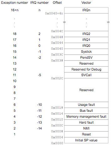Image source: section 2.3.4 of the Cortex-M4 Devices Generic User Guide

The first entry is the initial value of the stack pointer, and here we’re initialising it to __stack_end__. Setting the initial value of the stack pointer to the end of the stack rather than the beginning may seem counterintuitive, but keep in mind that adding something to the stack decrements the stack pointer, moving it to a lower value. The value of __stack_end__ is set by the linker script, and imported into this file by the .extern __stack_end__ statement near the beginning of the file. The linker script is a topic for a whole other post, but it is worthwhile mentioning that it’s responsible for making sure the exception vector table ends up in the right place in our firmware binary, so that it ends up in the right place in memory on the device when we flash our program on to it.

(If, like me, you’re a bit rusty on what the stack pointer is and how it is used, this page has a good explanation. It talks about the MIPS architecture, but the concepts are the same for ARM and pretty much every other processor architecture.)

Next up, in the second entry (memory offset 0x0004), is the reset vector. The reset vector is a pointer to the first instruction the processor should execute when it is reset. In our case, this is _start. We’ll come back to _start in a second.

The following entries give the addresses of various interrupt handlers. ARM calls them exception vectors, hence the name ‘exception vector table’. The first few handle failure scenarios, and then the rest cover the interrupts we’re used to dealing with, such as timers. I’m not going to go into too much detail here about this here, but Philip has defined a handy IRQ macro to use to help set these up. This enables us to define handlers only for the interrupts we’re interested in – if we don’t set up a handler for a particular interrupt, it’ll use a default handler that just returns immediately.

Step 2: preparation for user code: _start

So once the processor has initialised the stack pointer with __stack_end__, it starts executing the code specified in the reset vector. As we saw before, in our case, this is _start. Philip has done a pretty good job of explaining each instruction here, so I’m not going to go through it line by line, but I will call out the rough steps:

1. copy_data and copy_data_loop: Copy anything in the .data segment from flash to RAM. The .data segment includes global and static variables that have a non-zero initial value.

2. zero_bss and zero_bss_loop: Similar to the previous step, this initialises global and static variables that have a zero initial value in what is called the .bss segment. Why are zero values handled separately to non-zero values? It saves flash memory space, and is quicker to load: it takes much less space to store that X zero values are needed and initialise that many locations to zero than it does to record zero X times and then copy all those zeroes from flash into RAM.

   (Wikipedia and this page both have good explanations of the .data and .bss segments if you want to read more.)

3. call_ctors and ctors_loop: This does what the name suggests – it calls constructors for static and global variables.

4. run: The final step before we run our main() method is to call SystemInit(). SystemInit() is a function in system_stm32f4xx.c that sets up the processor’s clock. ST provides a utility to generate this file based on your application’s requirements and hardware. (The one I’m using should be suitable for the Discovery board.)

Step 3: main()

At this point, run branches to main() and we’ve finally made it! Everything has been initialised and the processor is running our code, happily doing whatever we’ve asked of it, whether that be flashing LEDs or controlling a chainsaw-wielding drone.

Step 4: life after main()

In most applications, main() is the last stop on our journey: it will usually eventually loop forever or put the microcontroller to sleep, and so main() will never return. However, we still need to handle the case where it does return.

If it does return, the processor will execute the next instruction after the call to main():

run: 
    ...other stuff in run

    bl     main                         // Call C main()
    // What's next?

If we don’t put something there, the processor could do anything – that memory location could potentially contain anything if we don’t explicitly set it to something. In our case, I’ve added an infinite loop:

run: 
    ...other stuff in run

    bl     main                         // Call C main()
    // Fallthrough

loop_if_end_reached:
    b      loop_if_end_reached          // Loop forever

References

• Whirlwind Tour of ARM Assembly
• Cortex-M4 Devices Generic User Guide, section 2.3.4: Vector table
• ARM and Thumb-2 instruction set quick reference guide

I set myself a bit of a challenge recently: pull together a working toolchain for a microcontroller. I’ve always used environments automagically generated by tools or prepared by others and so it’s been a bit of a mystery to me – I wanted to dig into the details to understand what’s going on.

The result of this challenge is a project template for the STM32F4 Discovery board, which you can find on GitHub.

I picked the STM32F4 series as it’s a relatively popular MCU choice and has a low-cost development board in the form of the Discovery board. It’s also an ARM processor, so there are plenty of good tools and resources available. The project template should work for any part in the STM32F4 series, although a bit of tweaking of some configuration files may be needed.

It still has some rough edges, but it should be ready for use by people who aren’t me. It has everything you need to get started:

• a working CMake-based build system, which uses the GCC ARM toolchain to produce a firmware binary
• a build target to flash that binary using stlink
• the STM32F4 DSP and standard peripherals library, if you want to use that

• a sample app that will flash the LEDs in a pattern. Yes, that’s right, flashing LEDs:

  

You can grab the template from GitHub. If you run into any issues or have any suggestions, creating issues on the repository is the best way to get in touch.

I’m planning on writing up a few posts explaining some of the more interesting parts soon… stay tuned.

On a recent project, we were struggling with our integration test suite. A full run on a developer PC could take up to 15 minutes. As you’d expect, that was having a significant impact on our productivity.

So we decided to investigate the issue and quickly discovered that the vast majority of that 15 minutes was spent spinning up and then destroying test databases for each test, rather than executing the tests themselves. (In the interests of test isolation, each individual test was given its own fresh database.) We didn’t want to stop giving each test a clean database, because we liked the independence guarantee that gave us, but at the same time, a 15 minute test run was well past the point of being bearable. There had to be a better way…

Some context

We were using SQL Server and the database schema we were testing against was a behemoth that had grown over many years to contain somewhere around 50 to 100 tables, plus dozens of stored procedures, views and indices. Creating a new database from scratch with this schema took 15-30 seconds.

Our production environment had nearly 1 TB of data, with most of that concentrated in two key tables that we frequently queried in different ways. As you can imagine, achieving an acceptable level of performance with this volume of data was challenging at times. (Thankfully we didn’t need that much data for each test.)

Because of this, we had a large amount of hand-crafted, artisanal SQL and were using Dapper. We had previously been using Fluent NHibernate to construct our queries, but found that NHibernate introduced a significant performance penalty which was not acceptable in our case. Furthermore, many queries involved a large number of joins and conditions that were awkward to express using the fluent interface and often resulted in inefficient generated SQL. They were much more expressive, concise and efficient in hand-written SQL.

Furthermore, some parts of the application wrote to the database, and different tests required different sets of data, so we couldn’t have one read-only database shared by all tests. Due to the number of database interactions under test and the number of tests, we wanted something that would have a minimal impact on the existing code.

The existing solution

The existing test setup looked like this:

1. Restore database backup with schema and base data
2. Insert test-specific data from CSV files
3. Run test
4. Destroy test database
5. Repeat steps 1 to 4 for each test

Apart from the performance issue I’ve already talked about, we also wanted to try to address some of these issues:

• The database was created from a backup stored on a shared network folder, meaning anyone could break the tests for everyone at any time. Moreover, it wasn’t under source control, so we couldn’t easily revert back to an old version if need be.

• The database was a binary file that was not easy to diff, which made it difficult to work out what had changed when tests suddenly started breaking.

• Any schema changes that were made needed to be manually applied to the database backup file (applying any new database migrations was not included in the test set up process). This meant tests weren’t always running against the most recent version of the schema.

What are snapshots?

Before we jump into talking about how we improved the performance of our tests, it’s important to understand SQL Server’s snapshot feature. Other database engines have similar mechanisms available, some built-in, some relying on file system support, but we were using SQL Server so that’s what I’ll talk about here. (Snapshots are unrelated to other things with the word ‘snapshot’ in them, such as snapshot isolation.)

Snapshots are just a read-only copy of an existing database, but the way in which they are implemented is critical to the performance gains we saw. Creating a snapshot is a low-cost operation as there is no need to create a full copy of the original database on disk. Instead, when changes are made to the original database, the affected database pages are duplicated on disk before those changes are applied to the original pages.

Then, when the time comes to restore the snapshot, it is just a matter of deleting the modified pages and replacing them with the untouched copies made earlier. And the fewer changes you make after the snapshot, the faster it is, as fewer pages need to be restored. This means that the act of restoring the database from a snapshot is very, very fast, and certainly much faster than recreating the database from scratch. This makes them well suited to our needs – we were recreating the database to get to a known clean state before the start of each test, but this achieves the same effect in much less time.

(If you’re interested in learning more, there are more details about how snapshots work and how to use them on MSDN.)

Introducing snapshots into our test process

After a few iterations, we arrived at this point:

1. Create empty test database
2. Run initial schema and base data creation script
3. Apply any migrations created since the initial schema and data script had been created
4. Take a snapshot of the database
5. Restore database from snapshot
6. Insert test-specific data from CSV files
7. Run test
8. Repeat steps 5 to 7 for each subsequent test
9. Destroy snapshot and test database

While this approach might be slightly more complicated, it gave us a huge performance boost (down to around 8 minutes). We were no longer spending a significant amount of time creating and destroying databases for each test.

There are a few other things of note:

• Step 5 (restoring the database from the snapshot) isn’t strictly necessary for the first test. We left it there anyway, instead of moving it to after running the test, just to make it clear that each test started with a clean slate. Also, as I mentioned earlier, the cost of restoring from a snapshot is negligible, especially when there are no changes, so this does not significantly increase the run time of the test.

• We addressed our first two ‘nice to haves’ by turning the binary database backup into an equivalent SQL script that recreated the schema and base data (used in step 2), and put this file under source control. Running the script rather than restoring the backup was marginally slower, but we were happy to trade speed for maintainability in this case, especially given that we’d only have to run the script once per test run.

• Step 3 (running any outstanding migrations) addressed the final ‘nice to have’. We couldn’t just build up the database from scratch with migrations because for some of the earliest parts of the schema, there weren’t any migration scripts. Also, we found that building a minimal schema script (and leaving the rest of the work to the migrations we did have) was a time-consuming, error-prone manual process.

Adding a dash of parallelism

Despite our performance gains, we still weren’t satisfied – we knew we could do even better. The final piece of the puzzle was to take advantage of NUnit 3’s parallel test run support to run our integration tests in parallel.

However, we couldn’t just sprinkle [Parallelizable] throughout the code base and head home for the day. If we did that without making any further changes, each test running at the same time would be using the same test database and would step on each other’s toes. We didn’t want to go back to having each test create its own database from scratch either though, because then we’d lose the performance gains we’d achieved.

Instead, we introduced the concept of a test database pool shared amongst all testing threads. The idea was that as each test started, it would request a database from the pool. If one was available, it was returned to the test and it could go ahead and run with that database. If there weren’t any databases available in the pool, we’d create one using the same process as before (steps 1 to 4 above) and then return that database. At the end of the test, it would then return the database to the pool for other tests to use.

This meant we created the minimum number of test databases (remember that creating the test database was one of the most expensive operations for us), while still realising another significant performance improvement – our test run was now down to around 5 minutes. While this still wasn’t as fast as we’d like (let’s be honest, we’re impatient creatures, tests can never be fast enough), we were pretty happy with the progress we’d made and needed to start looking at the details of individual tests to improve performance further.

Other approaches that we tried and discarded

We experimented with a number of other approaches that we chose not to use, but might work in other situations:

• Using a lightweight in-process database engine (eg. SQL Server Compact or SQLite), or something very quick to spin up (eg. Postgres in a Docker container): while this option looked promising early on, we needed to use something from the SQL Server family so that we were testing against something representative of the production environment, which left SQL Server Compact as the only option. Sadly, SQL Server Compact was missing some key features that we were using, such as views, which instantly ruled it out. (There’s a list of the major differences between Compact and the full version on MSDN.)

• Wrapping each test in a transaction, and rolling back the transaction at the end of the test to return the database to a known clean state: if we were writing our system from scratch, this is the approach I’d take. However, we already had a large amount of code written, and it would have been very time-consuming to rework it all to support being wrapped in a transaction. Most of the database code we had was responsible for creating a database connection, starting a transaction if needed and so on, and so reworking it to support an externally-managed transaction would have required a significant amount of work not only in that code but throughout the rest of the application.

• Using a read-only test database for code that made no changes to the test database: at one point in time, a large part of our application only read data from the database, so we considered having two different patterns for database integration testing: one for when we were only reading from the database, and another for when it was modified as part of the test (eg. commands involving INSERT statements). We shied away from this approach for the sake of having just one database testing approach.

Updated April 3: minor edits for clarity, thanks to Ken McCormack

Greg Skinner and I gave a presentation at Yow Connected in Melbourne on September 17, where we discussed how pairing can be a very effective form of collaboration for developers and designers.

The talk was recorded, so I hope there will be a video of it available soon. In the meantime, you can download a PDF version of the slides here.

The final version of the app we developed during the presentation is still live at http://yc.charleskorn.com, and the source code is also on GitHub.

I’ve been holding off posting about this because I was hoping the video would be posted, but it doesn’t seem to be coming… I’ll update this post if it does come out.

I gave a lightning / Pecha Kucha-style talk at DevOpsDays Melbourne on July 16 about our how we were able to deliver multiple production deployments a week at Trim for Life. This involved the use of (amongst other things) a microservices architecture, a backwards- and forwards-compatible data storage mechanism, fully automated deployment pipelines and automated monitoring.

The slides are available to download as a PDF.

Over the weekend I published two Ansible roles for automating common set up tasks for a Raspberry Pi:

• raspi-information-radiator: configures a Raspberry Pi as an information radiator, automatically launching Chromium to display a web page in full screen mode on boot. (This is based on the article HOWTO: Boot your Raspberry Pi into a fullscreen browser kiosk.)

• raspi-expanded-rootfs: expands the root filesystem of a Raspberry Pi to fill the available space.

They’re also available on Ansible Galaxy.

The readme files for both roles include more information on how they work and an example of how to use them.

Both of them have some opportunities for improvement, and pull requests and issue reports are most welcome.

The purpose of this post is to document what I’m using to run this blog (and thus serve as some kind of prompt when I’m trying to fix stuff in six months’ time) and hopefully also help you set up your own blog.

The tl;dr version: Jekyll + GitHub Pages + custom domain name = charleskorn.com

Hosting

I use GitHub Pages to host this blog. If you’ve never heard of GitHub Pages before, it is a completely free static website hosting service provided by GitHub. As you might expect with something coming from GitHub, each site is backed by a Git repository (mine is charleskorn/charleskorn.github.io, for example). This means you instantly get things like version history, backups and offline editing with zero extra effort.

You can use GitHub Pages to create a site for a user (which is what I have done for this site), a single repository or an organisation. More details on the differences are explained in the help area.

You can use it to host purely static content, or you can have your final HTML generated by the Jekyll static site generator, which is what I use. As soon as you push your changes up to your GitHub repository, all the static files are automatically regenerated within a matter of seconds.

With Jekyll, you write your posts as Markdown files, and then it generates HTML from your posts based on templates that you define. It also has built in SASS and CoffeeScript compilation, RSS feed generation and support for permalinks, amongst other things. It’s also straightforward to set up a custom 404 page.

Side note: as you can imagine, some features of Jekyll are restricted by GitHub. For example, there is a limited set of allowed plugins, but by and large, you can use the full functionality of the core Jekyll project. If you need more flexibility, you can always generate the pages yourself and push the result up to a branch called gh-pages, or just turn Jekyll processing off altogether. (We use this technique for the ThoughtWorks LevelUp website, for example.)

The final missing piece of the puzzle is setting up a custom domain name to point at the site hosted by GitHub. This is fairly straightforward to do. It requires creating a CNAME file in the root directory of your repository with the domain name you’d like your site to use (you can see mine for an example), and then configuring your DNS server to point at GitHub’s servers.

Writing process

My writing process looks something like this at the moment:

• bundle exec jekyll draft "My cool new article"
• bundle exec guard
• writing, checking a live preview in my browser
• procrastinating
• more writing
• editing and proofreading
• bundle exec jekyll publish _drafts/my-cool-new-article.md
• git commit -m "My cool new article"
• git push

Not all of this is built in to Jekyll:

The jekyll draft and jekyll publish commands come from a handy plugin called jekyll-compose. They don’t do anything you couldn’t do yourself – jekyll draft just sets up the scaffolding of a draft post and jekyll publish just moves that post into the _posts folder and adds the date to the file and the front matter – but they certainly make things that little bit easier.

There are a couple of things that work together to produce live previews in a browser. The guard-jeykll-plus plugin for guard makes use of Jekyll’s built-in auto-regeneration support to automatically regenerate the site when any change is detected. Once that’s done, the guard-livereload plugin sends a notification to a small JavaScript snippet embedded into every page to trigger a reload once the build process is finished.

SEO

I also used the opportunity of setting up this blog to learn about some standard SEO practices for websites (given the topic sometimes comes up in my day job).

The first thing was setting up Google Analytics (for traffic reporting and analysis) and Google Webmaster Tools (for alerts from Google when something goes awry). The easiest way to do this is to use Google Tag Manager. This makes it easy to manage all the necessary JavaScript tags for your site, and only requires a single JavaScript tag on your pages – the rest are inserted dynamically based on your configuration.

The next step was adding an XML sitemap, which helps search engines discover all of the pages on your site. This is can be generated for you as part of the Jekyll build process by the jekyll-sitemap plugin.

However, simply generating the sitemap isn’t enough – you also need to tell Google about it. You can use Webmaster Tools to do this instantly, or list it in your robots.txt and Google’s crawler will pick it up next time it indexes your site. Furthermore, when the content on your site changes, it’s a good idea to ping Google to let it know. I have a Travis CI job set up to do this automatically whenever I push changes to GitHub. (This also checks for simple issues like broken links and malformed HTML using html-proofer.) It’s a similar process for other search engines as well.

Another thing that I’m not 100% sold on the value of is schema.org markup. The idea is that you decorate your HTML with extra attributes that describe what their content means, for example, that a span contains the author’s name, or that a h2 is the blog post title. It enables some of the extra information you sometimes see next to search results such as the date the post was written and the author’s name, but I’m not sure how much it helps with people actually finding content relevant to their query. (Although I’m sure that if Google told us that it did impact search ranking, you can bet that it would be exploited within hours, diminishing its usefulness somewhat.)

This turned out to be much longer than I expected… I hope you found this useful (even if this is just Future Charles reading this).

Following on from my previous blog post about rkt, I’ve published an Ansible role I use to deploy a simple systemd service unit that runs an ACI (the image format used by rkt).

You can find it on Ansible Galaxy at https://galaxy.ansible.com/list#/roles/3736, and on GitHub at https://github.com/charleskorn/rkt-runner.

Like the previous post, this written for the v0.5.5 release of rkt, so some things may be slightly outdated.

This post was written for the v0.5.5 release of rkt, so some things may be slightly outdated.

I’ve recently been experimenting with rkt (pronounced ‘rock-it’), a tool for running app containers. rkt comes from the team at CoreOS, who you might know from other projects such as etcd and fleet. rkt is conceptually similar to Docker, but was developed by CoreOS to address some of the shortcomings they perceive in Docker, particularly around security and modularity. They wrote up a great general overview of their approach in the rkt announcement blog post.

I was initially drawn to rkt because of the difficulty running Docker on a Raspberry Pi without recompiling the kernel. (Although, as of now, I still haven’t got rkt running on it either - that should change soon though, see below.)

My goal with this blog post is to discuss some of the things I’ve liked about rkt, and some of the frustrations.

Image build process

The first thing that struck me about rkt was the simplicity and speed of the image build process. A simple image for a personal project takes four seconds to build, and most of that is spent compiling the Golang project that makes up the image. (This is the shell script that I use to compile that image if you’re interested.) This simplicity and speed stems from the fact that neither the image nor its base image (if there is one) are actually started during the build process when using the standard build tool (actool). Instead, each image is created from the files it requires and a list of images it depends on to run. Not booting the container also eliminates the need to download the base images to the build machine, saving further time. Moreover, the runtime provides a standard base image upon which all other images are run (called the stage 1 image), eliminating the need for a base image in many simple cases. (Similar to Docker, the “merging” of the top-level image with its dependencies happens at runtime, using overlayfs if available on the host.)

Removing the need to boot up an image during the build process also has some other advantages. It makes it far easier to run on different architectures or operating systems to those on the target machine. For example, it’s quite easy to build an image targeting Linux from OS X, and no tools like boot2docker are required. Furthermore, the build process can be run as an unprivileged (non-root) user, which can make life easier in restricted hosted build environments.

However, this approach does have one major drawback that can make life very painful. As the container is not booted, tools such as apt-get can’t be used to easily install dependencies - you’re responsible for ensuring that all dependencies find their way onto the image yourself. With a simple Golang server, for example, this isn’t a big issue, as it’s quite straightforward to produce a statically-linked binary, but for many other languages this can be problematic as the entire runtime and their dependencies are required (eg. a JVM, Ruby runtime etc.).

Separation of build tools and runtime

As I mentioned earlier, one of the major focus areas has been on modularity and enabling developers to use the most appropriate tool for the job, rather than the more one-size-fits-all approach of Docker. As such, the runtime (rkt) is completely separate from the build tool (actool), and either could be completely replaced by another tool - the specification they conform to is available on GitHub. There are already some alternative runtime implementations and a variety of different tools springing up.

Security / image verification model

One of the most interesting aspects of rkt is its security model. rkt comes with cryptographic verification of images enabled by default (and defaults to trusting no signing keys). This enables you to ensure that not only are public images are from those you trust, but also that any private images you upload to services outside your control are unmodified when you pull them back down again. It’s also pretty straightforward to set up and running, with a good guide available on GitHub.

Compatibility with Docker

Although I haven’t tried this myself, it’s possible to run Docker images with the rkt runtime, if you need to run both Docker and rkt images side-by-side. (source)

Documentation

rkt is still very much under active development - there have been 14 releases since the first at the end of November last year - which means what little documentation and online resources are out there are generally made obsolete very quickly, which can be a bit of a pain at times. There is a focus on stabilising things with the upcoming 0.6 release, but until that materialises, keep in mind that anything you’re reading now could be very out of date.

Furthermore, the official documentation is patchy - some places (such as the app container specification) are thorough, whilst other places are full of placeholders.

Multiple architectures

Because the stage 1 image is provided by the host environment, building images for different architectures is (theoretically) easier - if your image does not require a specific base image, all you need to do is recompile your binaries for the other architecture. (I say theoretically because I haven’t yet tried it myself - I’m still waiting for support for running containers on ARM processors, which is expected in the 0.6 release.)

Conclusion

I’ve really liked working with rkt so far - it’s been very quick to get up and running and there wasn’t a lot of fussing around to get something simple working, even in its current form. There are still some rough edges, particularly around documentation, and some things that can make life frustrating, like dealing with dependencies, but there is definitely a lot of potential. It’s going to be very interesting to watch rkt evolve.

Thanks for visiting… I’m going to try to post semi-regularly.